Chapter 8 — Price Elasticity, Income Elasticity, and Cross Elasticity of Demand
Cambridge International AS & A Level Economics (9708) · Unit 2.2 · 4th edition coursebook
Learning objectives
- Define price elasticity of demand (PED), income elasticity of demand (YED), and cross elasticity of demand (XED).
- Calculate each from data and interpret the value.
- Explain the determinants of PED, YED and XED.
- Link PED to total revenue and the slope of the demand curve.
Key terms
- price elasticity of demand (PED)
- The responsiveness of quantity demanded to a change in the good's own price, measured as %ΔQd / %ΔP.
- income elasticity of demand (YED)
- The responsiveness of quantity demanded to a change in consumer income, measured as %ΔQd / %ΔY.
- cross elasticity of demand (XED)
- The responsiveness of quantity demanded of one good to a change in the price of another, measured as %ΔQd(X) / %ΔP(Y).
- elastic demand
- |PED| > 1: a 1% price change causes a larger than 1% quantity change.
- inelastic demand
- |PED| < 1: a 1% price change causes a smaller than 1% quantity change.
- unit elastic demand
- |PED| = 1: a 1% price change causes a 1% quantity change. Total revenue does not change.
- perfectly elastic demand
- PED = ∞: a horizontal demand curve — any rise in price collapses quantity to zero.
- perfectly inelastic demand
- PED = 0: a vertical demand curve — quantity does not respond to price.
- luxury good
- A good with YED > 1: demand rises more than in proportion to income.
- necessity good
- A normal good with YED close to zero — demand changes only weakly with income.
8.1Price elasticity of demand (PED)
Price elasticity of demand measures how sensitive consumers are to a price change. By convention we take the absolute value: |PED| > 1 is elastic; |PED| < 1 is inelastic; |PED| = 1 is unit elastic.
Special cases include perfectly elastic demand (a horizontal curve, shown in Figure 8.4) and perfectly inelastic demand (a vertical curve, shown in Figure 8.3), as well as the borderline case of unit-elastic demand (a rectangular hyperbola, shown in Figure 8.5). On a downward-sloping straight-line demand curve, as in Figure 8.6, PED varies along its length — elastic at the top, inelastic at the bottom. Figure 8.2 illustrates the contrast: an inelastic product (such as Product A) shows a small response to a price change, while an elastic product (such as Product B) shows a large response to the same change.

Price-elastic demand means quantity demanded responds more than proportionately to a price change, so total revenue moves inversely with price. Option D – a price fall raising revenue – is the defining outcome: the percentage rise in quantity exceeds the percentage fall in price, lifting P x Q. Option A only describes any responsive demand, B describes the law of demand generally, and C contradicts elastic behaviour.
8.2Determinants of PED
Five main factors determine how elastic demand is:
- Availability of substitutes. Many close substitutes → elastic.
- Necessity vs. luxury. Necessities have inelastic demand; luxuries are elastic.
- Proportion of income. Items that take a small share of income (chewing gum) are inelastic; big-ticket items are elastic.
- Time horizon. Demand is more elastic in the long run as consumers adjust habits and find substitutes.
- Addiction / habit. Addictive goods (tobacco) tend to be inelastic.
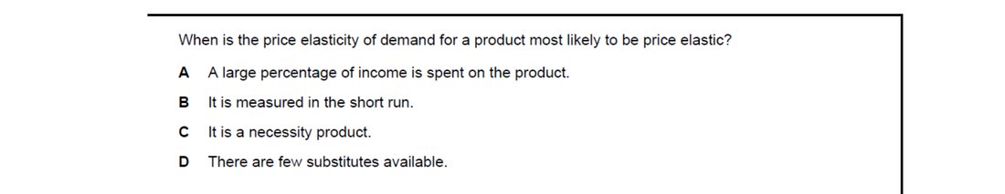
Demand is most price elastic when the good takes a large share of income, has many substitutes, is a luxury, or is judged over a long time period. Option A – a large percentage of income spent on the product – makes buyers especially sensitive to price changes, so they adjust quantity strongly. Options B, C and D all point toward inelastic, not elastic, demand.
8.3PED and total revenue
Total revenue = price × quantity. When demand is elastic, a price cut raises total revenue (and a price rise reduces it) because the percentage increase in quantity exceeds the percentage cut in price. When demand is inelastic, a price rise raises total revenue. At unit elasticity, total revenue is at a maximum and unchanged by small price moves.
Figure 8.9 contrasts an elastic and an inelastic demand curve passing through the same point. The same $1 price rise produces a much larger quantity fall on De than on Di — and therefore a different revenue effect. Figure 8.10 then traces the consequences for total revenue: (a) inelastic demand — a price rise raises revenue; (b) elastic demand — a price cut raises revenue.
This is the central pricing insight in the syllabus: a firm's optimal price depends on the elasticity of demand it faces. Figure 8.8 applies the same idea to a real market — a change in demand for PCs — illustrating how the elasticity of the demand curve shapes the price and quantity response.
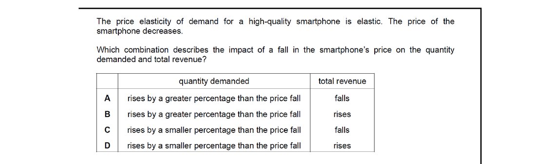
Elastic demand means %change in Q exceeds %change in P. When price falls, quantity rises by a larger percentage, so total revenue (P x Q) rises. Option B captures both effects: quantity demanded rises by a greater percentage than the price fall, and total revenue rises. Options A and C wrongly predict falling revenue; D understates the quantity response.
8.4Income elasticity and cross elasticity
Income elasticity of demand classifies goods, as summarised in Figure 8.7. YED > 1 → luxury. 0 < YED < 1 → necessity. YED < 0 → inferior good.
Cross elasticity of demand reveals the relationship between two goods. XED > 0 indicates substitutes (a rise in P(Y) raises Qd(X)); XED < 0 indicates complements (a rise in P(Y) reduces Qd(X)); XED = 0 indicates unrelated goods.
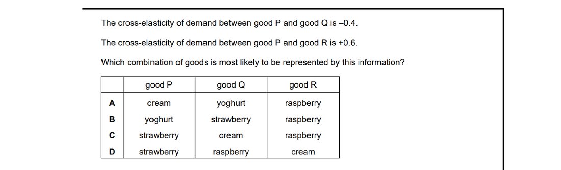
Cross elasticity is negative for complements and positive for substitutes. With XED(P,Q) = -0.4 (complements) and XED(P,R) = +0.6 (substitutes), P must pair naturally with Q and rival R. Option C – strawberry (P), cream (Q, complement), raspberry (R, substitute) – fits both signs, since cream is consumed with strawberries while raspberries compete with strawberries.
End-of-chapter practice
Past-paper questions from CIE 9708. Pick A, B, C or D. Answers are saved on this device — press Download report (PDF) at the top to save them.
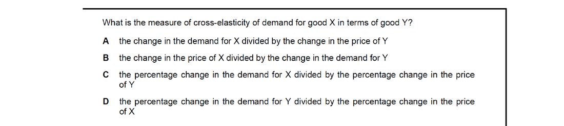
Cross elasticity of demand measures the responsiveness of demand for one good to the price of another, expressed as percentage changes. Option C – %change in demand for X divided by %change in price of Y – is the textbook formula. Options A and B use absolute changes rather than percentages, and D reverses the goods, giving XED of Y with respect to X.
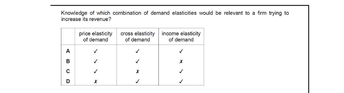
Revenue depends on price (via PED), competitors' prices (via XED) and consumer incomes (via YED). A firm aiming to raise revenue benefits from knowing all three elasticities, so it can set price, respond to rivals and anticipate income-driven demand shifts. Option A – all three elasticities relevant – is therefore correct; the other rows omit at least one essential piece of information.
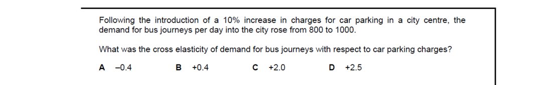
Cross elasticity = %change in demand for bus journeys / %change in car-parking charges. Bus demand rises from 800 to 1000, a 25% increase, while car-parking charges rise 10%. XED = +25/+10 = +2.5, positive because the two services are substitutes. Option D matches this calculation; A and B miscompute the sign or magnitude, and C uses 20% instead of 25%.
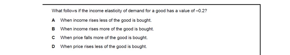
Income elasticity of demand = %change in quantity demanded / %change in income. A negative YED of -0.2 marks an inferior good: as income rises, quantity demanded falls. Option A – when income rises less of the good is bought – states exactly this. Options C and D wrongly involve price changes (PED, not YED), and B describes a normal good.
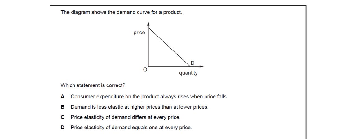
Along a straight-line, downward-sloping demand curve PED varies continuously: elastic on the upper half, unit-elastic at the midpoint and inelastic on the lower half. Option C – PED differs at every price – captures this. Option A is false where demand is inelastic, B reverses the relationship, and D would only hold for a rectangular hyperbola, not a straight line.
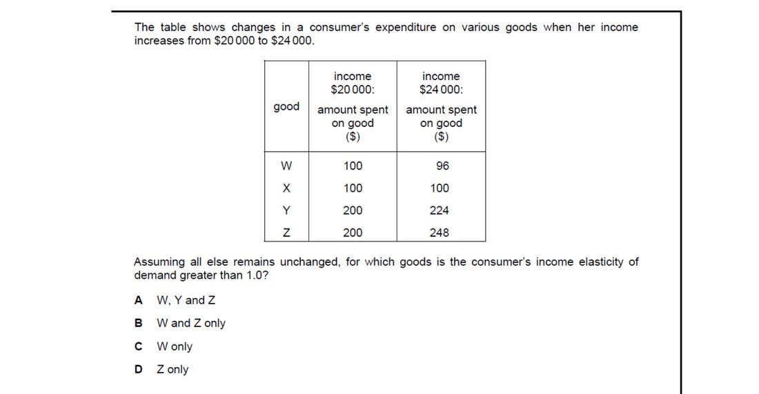
YED > 1 identifies a luxury: spending rises proportionately faster than income. Income rises 20% ($20000 to $24000). For W spending falls (YED negative), X is unchanged (YED = 0), Y spending rises 12% (YED = 0.6, below 1), but Z rises 24% giving YED = 1.2 > 1. Only good Z qualifies, so option D is correct.
Attempt the practice questions above to build your score.
Self-evaluation checklist
After studying this chapter, you should be able to:
- Calculate PED, YED and XED from data and interpret the values.
- Identify what makes demand elastic or inelastic.
- Predict how a price change affects total revenue using PED.
- Use YED to classify goods; use XED to identify substitutes and complements.
Want more practice? Drill this chapter's past-paper MCQs (117 questions) →